If you have any questions about this post please ask on the discussion thread on /r/machinelearning.

For a solid introduction to Automatic Differentiation, which is the subject of this blog post, see Automatic differentiation in machine learning: a survey.

Last week I was involved in a heated discussion thread over on the Autograd issue tracker. I’d recently been working on an implementation of forward mode automatic differentiation, which fits into Autograd’s system for differentiating Python/Numpy code. Our discussion was about the usefulness of forward mode, which is equivalent to Theano’s Rop and in the general case is used to calculate directional derivatives, or equivalently for calculating Jacobian vector products.

Reverse mode automatic differentiation (also known as ‘backpropagation’), is well known to be extremely useful for calculating gradients of complicated functions. In the general case, reverse mode can be used to calculate the Jacobian of a function left multiplied by a vector. In the thread linked above, and in the Autograd codebase, any function which does this reverse mode vector-Jacobian product computation is abbreviated to vjp. The usefulness of a vjp operator, which takes a function as input and returns a new function for efficiently evaluating the original function’s vjp, is clearly beyond dispute — the familiar grad operator $\nabla$ is a special case of such an operator. Such operators have now been implemented in different forms in many many machine learning software packages: TensorFlow, Theano, MXNet, Chainer, Torch, PyTorch, Caffe… etc etc.

But how useful are the Jacobian-vector products (or jvps, as opposed to vjps), which are calculated by forward mode (as opposed to reverse mode), particularly in machine learning? Well they may be useful as a necessary step for efficiently calculating Hessian-vector products (hvps), which in turn are used for second order optimization (see e.g. this paper), although as I was arguing in the thread linked above, in an idealised implementation you can obtain an equivalent hvp computation by composing two reverse mode vjp operators (Lops in Theano).

Later in the thread we were discussing another very specific use case for forward mode, that of computing generalised Gauss Newton matrix-vector products, when we happened upon a new trick: a method for calculating jvps by composing two reverse mode vjps! This could render specialised code for forward mode redundant. The trick is simple. I’ll demonstrate it first mathematically and then with Theano code.

The trick

Firstly, note that our reverse mode operator takes a function as input and returns a function for computing vector-Jacobian products. In mathematical notation, if we have a function

$$f:\mathbb{R}^m \rightarrow \mathbb{R}^n$$

then

$$\mathrm{vjp}(f)(v, x) = v^\top \frac{\partial f}{\partial x}(x)$$

where $\frac{\partial f}{\partial x}$ is shorthand for the Jacobian matrix of $f$:

$$\frac{\partial f}{\partial x} = \begin{bmatrix} \frac{\partial f_1}{\partial x_1}&\cdots&\frac{\partial f_1}{\partial x_m}\\ \vdots&\ddots&\vdots\\ \frac{\partial f_n}{\partial x_1}&\cdots&\frac{\partial f_n}{\partial x_m} \end{bmatrix}.$$

Now if we treat $x$ as a constant, and consider the transpose of the above, which I will denote $g$, we have

$$g(v) = \left[\mathrm{vjp}(f)(v, x)\right]^\top = \left[\frac{\partial f}{\partial x}(x)\right]^\top v.$$

Note that $g$ is a linear function of $v$. The Jacobian of $g$ is therefore constant (w.r.t. $v$), and equal to $\left[\frac{\partial f}{\partial x}(x)\right]^\top$, the transpose of the Jacobian of $f$.

So what happens when we apply the vjp operator to $g$? We get

$$\begin{align} \mathrm{vjp}(g)(u, v) &= u^\top \frac{\partial g}{\partial v}(v) \\ &=u^\top\left[\frac{\partial f}{\partial x}(x)\right]^\top \\ &=\left[ \left[ \frac{\partial f}{\partial x}(x)\right] u \right]^\top \end{align}$$

The Jacobian of $f$ is being right-multiplied by the vector $u$ inside the bracket, and taking the transpose of the whole of the above yields

$$\left[\mathrm{vjp}(g)(u, v)\right]^\top = \left[ \frac{\partial f}{\partial x}(x)\right] u,$$

the Jacobian of $f$ right multiplied by the vector $u$ — a Jacobian-vector product.

Example implementation with Theano

In Theano the jvp operator is theano.tensor.Rop and the vjp operator is theano.tensor.Lop. I’m going to implement an ‘alternative Rop’ using two applications of theano.tensor.Lop, and demonstrate that the computation graphs that it produces are the same as those produced by theano.tensor.Rop.

Firstly import theano.tensor:

import theano.tensor as T

and let’s take a quick look at the API for Rop, which we’ll want to copy for our alternative implementation:

T.Rop?

Signature: T.Rop(f, wrt, eval_points)
Docstring:
Computes the R operation on `f` wrt to `wrt` evaluated at points given
in `eval_points`. Mathematically this stands for the jacobian of `f` wrt
to `wrt` right muliplied by the eval points.

The important thing here is: T.Rop(f, wrt, eval_points) stands for ‘the jacobian of f wrt to wrt right muliplied by the eval points’. So wrt was what I denoted $x$ above, and eval_points was denoted $u$.

I prefer my notation, so I’m going to use x and u for those variables. The signature of our alternative_Rop is going to look like this:

def alternative_Rop(f, x, u):

The theano.tensor.Lop API matches that of Rop. So T.Lop(f, wrt, eval_points) evaluates the Jacobian of f with respect to wrt, left multiplied by the vector eval_points. Carefully tracing through the equations above, we can implement our alternative Rop. It’s pretty simple:

def alternative_Rop(f, x, u):
    v = f.type('v')       # Dummy variable v of same type as f
    g = T.Lop(f, x, v)    # Jacobian of f left multiplied by v
    return T.Lop(g, v, u)

Note that we don’t need any transposes because the output of Theano’s Lop actually comes ready transposed.

Let’s test this out on a real function and check that it gives us the same result as Theano’s default Rop. Firstly define an input variable and a function:

x = T.vector('x')
f = T.sin(T.sin(T.sin(x)))

and a variable to dot with the Jacobian of f

u = T.vector('u')

Then apply the original Rop and our alternative:

jvp = T.Rop(f, x, u)
alternative_jvp = alternative_Rop(f, x, u)

and compile them into Python functions

import theano
jvp_compiled = theano.function([x, u], jvp)
alternative_jvp_compiled = theano.function([x, u], alternative_jvp)

Then evaluate the two functions to check they output the same thing:

import numpy as np

x_val = np.random.randn(3)
u_val = np.random.randn(3)

jvp_compiled(x_val, u_val)

array([-2.17413113, -0.02833015, -0.08724173])

alternative_jvp_compiled(x_val, u_val)

array([-2.17413113, -0.02833015, -0.08724173])

The different versions seem to be doing the same computation, now to look at their computation graphs.

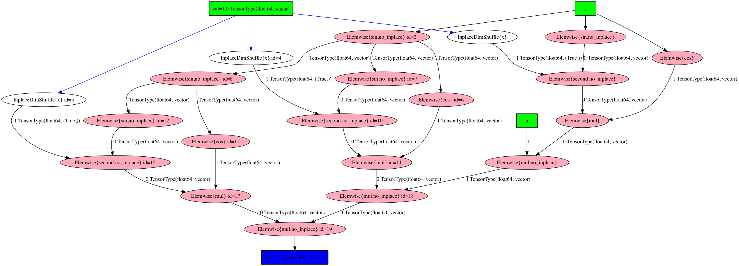
Firstly the default Rop

from IPython.display import Image
display(Image(theano.printing.pydotprint(jvp, return_image=True, var_with_name_simple=True)))

and our alternative Rop

display(Image(theano.printing.pydotprint(alternative_jvp, return_image=True, var_with_name_simple=True)))

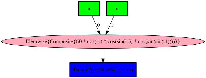
The pre-compilation graphs above appear to have the same chain-like structure, although the graph produced by the alternative Rop actually looks a lot simpler (whether this is something that would happen for general functions I do not know). Notice the variable v doesn’t appear in the alternative Rop graph — Theano recognises that it’s irrelevant to the final computation. After compilation the graphs appear to be exactly the same (albeit with the positions of the u and x nodes swapped):

display(Image(theano.printing.pydotprint(jvp_compiled, return_image=True, var_with_name_simple=True)))

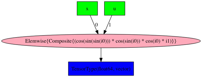
display(Image(theano.printing.pydotprint(alternative_jvp_compiled, return_image=True, var_with_name_simple=True)))

Conclusions and notes

Assuming the behavior above generalises to other Theano functions, it looks like much of the code implementing Rop in Theano may be unnecessary. For Autograd, the situation isn’t quite as simple. Autograd doesn’t do its differentiation ahead of time, and needs to trace a function’s execution in order to reverse-differentiate it. This makes our new trick, in its basic form, significantly less efficient than the forward mode implementation that I’ve written.

Some more discussion and a TensorFlow implementation can be found on the tensorflow-forward-ad issue tracker. It’s quite likely that our ‘new’ trick is already known within the AD community, please email me if you have a reference for it and I will update this post.